Interpolation.xla (with new functions)
In this page you can download an Excel Add-in useful to linear, quadratic and cubical interpolation and extrapolation.
The functions of this Add-in are very simple to use and they have context help, through a chm file.
![]()
If you have an old release of Interpolation.xla, delete it, save the new file and seek it from Excel | "File" or "Microsoft Office Button" | "Excel Options" | Add-Ins | Go. Browse and Charge it again. You'll see a prompt to permit the replacement. Do the same in case of your first time with this Add-in.
Release 2.0 April 6th 2016 for Excel 2010, 2013 and higher versions running in Windows 7 and Windows 10.
Release 2.1 February 2020.
You can also download a pdf file: InterpolationV2.pdf
Once downloaded and unzipped, you will see two files. You have to move Interpolation.chm to the following folder:
C:\Program files\Microsoft Office\Root\Office16\Library or:
C:\Program files\Microsoft Office\OFFICE15\Library (You can see the correct path in "Trusted Locations" of "Trust Center")
But, previously you have to change properties of "Interpolation.chm" because Windows blocks this type of files when they are downloaded from the Internet, as it does with other types of files, for example, xls files. If you do not do this, help with functions will not be available.
File Interpolation.xla can be placed in any folder but could be better moving it to the folder where Excel looks for Add-ins.
Old version 1.09 (help via chm file) It works fine with Excel 2007 and Windows XP, W7
Old version 1.08 (help via hlp file) It works fine with Excel 2003 and Windows XP
If you do not want to use VBA code but only using normal Excel functions see this page
Working with Interpolation.xla
CERCHA
(X;Range_xy;"Keys";V1;V2)
____________________________________________________
Required arguments: X;Range_xy
Optional arguments: "Keys";V1;V2
(see explanation of optional
arguments)
Important: the
positions and the separators must be respected (";" or "," according to Excel
or Windows configuration ).
This function
is used for interpolation or extrapolation using splines. Splines are cubic
polynomial functions that adapt by pieces to the points where you have to
interpolate, in such a way that between pairs of contiguous points there are
different polynomials (with exceptions). The derivative slope and second
derivative at the ends of the splines, match with the next spline and the
values at the start of first and the end of the last splines can be make up on
the basis of the type of spline that is needed, that is to say, settle down
"end-point constraints".
Important: Data must be ordered in ascending and the end-point constraints will
be applied, first (1st key and v1) for the smaller value of Range_xy (column 1) and
(2nd key and v2) for the greater value of Range_xy (column 1).
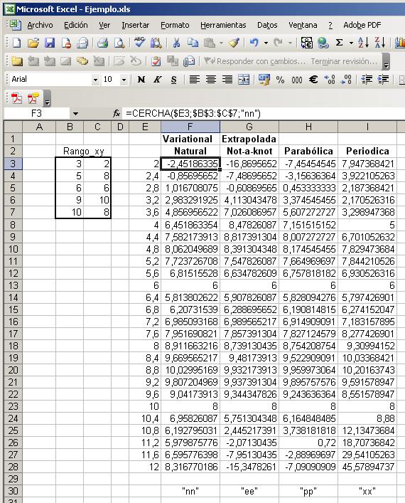
Example of use of the function CERCHA
In this example we are going to work with a cubic spline. The spline has a forced condition
at the first and last point (slope -1.5 and 1.5).
It is a Clamped spline
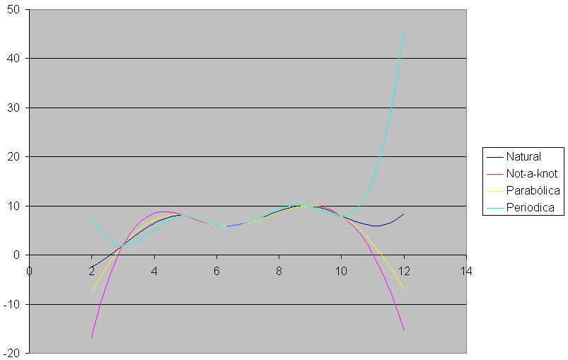
Plot of the spline and interpolation at x= 3.5
Here you can see the first and last slopes
Interpolation.xla Functions
Linear
Interpolation:
Cubic Interpolation:
CERCHA Cubic spline interpolation.
CERCHAC Spline coefficients.
CERCHACOEF
Spline coefficients (ref. axis origin).
CERCHAP Slope in well-known data.
CERCHAPI Initial slope at the first spline.
CERCHAPF Final slope at the last spline.
CERCHACI Initial second derivative of the first spline.
CERCHACF Final second derivative of the last spline.
CERCHARA Curvature radii at well-known data.
CERCHARAXY Centre
of curvature coordinates.
CERCHACU Second derivatives at well-known data.
CERCHACUR Curvature at points.
CERCHAREA Area under the spline.
CERCHAMX Statical moment respect X axis.
CERCHAMY Statical moment respect Y axis.
CERCHAM2X Second moment (inertia) respect X axis.
CERCHAM2Y
Second moment (inertia) respect Y axis.
CERCHAP2 Product of inertia.
CERCHAXG Centre of gravity Xg.
CERCHAYG Centre of gravity Yg.
CERCHALON Lenght of chord of spline.
New functions:
CERCHAK Akima spline (stable to the outliers).
CERCHAKCO Akima spline coeffcients.
CERCHAKD Akima spline first and second derivatives.
CERCHAKIN Akime spline integration.
CERCHAS Cubic spline interpolation (Alglib algorithm).
CERCHASCO Spline coefficients.
CERCHASD First and second derivatives.
CERCHASIN Spline integration.
CERCHAH Hermite spline interpolation.
CERCHAHCO Hermite spline coefficients.
CERCHA2D Hermite spline second derivative.
CERCHAHIN
Hermite spline integration.
Example of interpolation in the stability curve of a ship
Initial data:
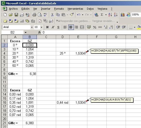
The word "Escora" means: Heel
GMc: Metacentric height corrected for free surfaces effect
Due to the corrected Metacentric height matches up with the slope of the stability curve at origin and at the end of the curve it matches with zero curvature line (straight line), we can use the following end-point constraints for the spline: fn
f forced spline (clamped spline)
n natural or variational spline
In Cell E4 formula we can see that the value is multiplied by "PI()/180". This is because heel has to be expressed in radians.
1 radian =180/PI() = 180 / 3.14159 = 57.296 degrees
Here you can see several interpolations. You can export the data, for example to Autocad
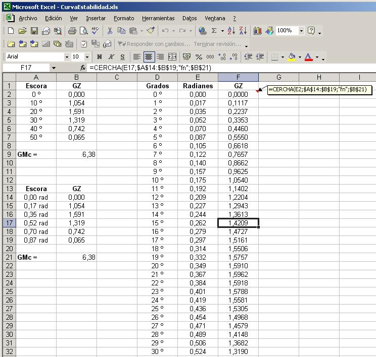
You can convert Range_xy in an absolute reference by pressing F4. It is important to avoid the change of data in the argument Range_xy when you copy the formula. The same tip is for the data of GMc. To avoid working with references and Ranges you can insert (assign) a name for a specific Range or cell and use it as an argument in the formulas.
Excel® has a Graphic assistant but if you like export data to Autocad®, you can do the following procedure:
At first you have to copy the x and y data of a curve to a new sheet.
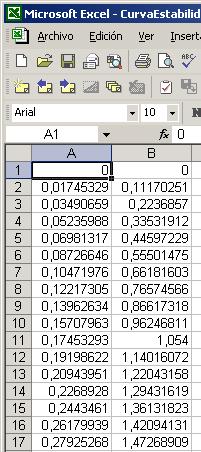
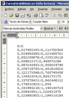
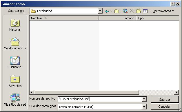
Save it with CSV format (use quote and write scr as file extension for example "CurvaEstabilidad.scr"). Then edit it with Word® changing the decimal point of the file or argument separator using replace in Edit menu. Finally, add up a line with the Autocad order for a polyline.
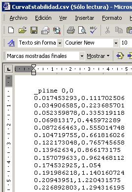
Now we have an script file for Autocad. In Autocad we can use Run script and the curve will be done.

Use of several end-point constraints
Plot of the splines
Interpolation example in the hydrostatic table of a ship using INTERPO
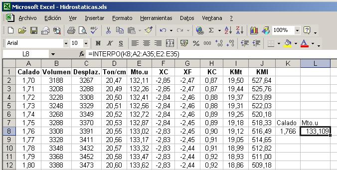
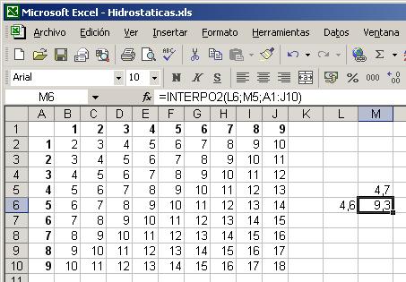
Double linear interpolation
March 31st 2022